Strong FBG, Weak FBG, or Fully Distributed: Choosing Among the Three Fiber-Optic Sensing Routes
Fiber-optic sensing has been discussed in the structural monitoring community for more than twenty years, yet the first question on a real project is usually not "should we use fiber" but "which kind of fiber". Strong-reflection gratings, weak-reflection gratings and fully distributed sensing are all called fiber-optic sensing, but their price, accuracy, point count and installation practice differ by more than an order of magnitude. Choose the wrong route, and every later decision — bonding technique, interrogator, data interpretation — becomes an uphill battle.
This article skips the textbook introduction and goes straight to the physics that separates the three routes, what each is good at, and what typically goes wrong in the field.
The Common Foundation: How Light "Senses" Inside a Fiber
All three technologies rest on the same fact: light traveling in a fiber is modified by the outside world.
For grating-based sensors, the quantity being modified is the wavelength. A fiber Bragg grating (FBG) is a periodic modulation of the refractive index written into the fiber core. Light satisfying the Bragg condition is reflected, with center wavelength λB = 2·n_eff·Λ (n_eff is the effective refractive index, Λ the grating period). Strain lengthens Λ and temperature changes n_eff, so the reflection peak shifts. Around 1550 nm the typical sensitivities are about 1.2 pm/με for strain and about 10 pm/℃ for temperature — meaning 100 microstrain moves the peak by only 0.12 nm. That is an extremely fine signal, and a very fragile one.
For distributed techniques, the modified quantity is a parameter of the scattered light: the phase of Rayleigh backscatter (vibration/acoustics), the Brillouin frequency shift (temperature and strain), or the Raman intensity ratio (temperature only). There is no grating — the fiber itself is the sensor, continuously along its entire length.
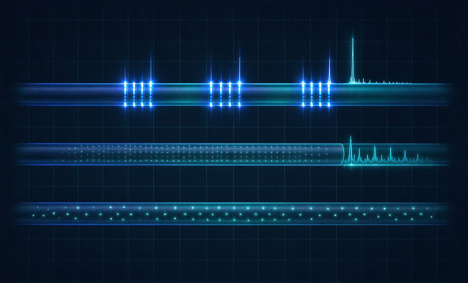
With that in mind, the dividing line among the three routes becomes clear: gratings are "discrete points", distributed sensing is "continuous with no points at all". And the difference between strong and weak reflection is essentially "how many points can you fit on one fiber".
Strong-Reflection Gratings: Highest Accuracy, Fewest Points
A conventional FBG has a reflectivity of roughly 50%–90%, returning a narrow, clean spectral peak.
Why strong reflection works well: the reflected optical power is ample, so the interrogator only needs a broadband source plus a wavelength-scanning mechanism or tunable filter. Signal-to-noise ratio is high, wavelength resolution reaches the 1 pm level, which translates to strain resolution better than 1 με — the highest accuracy of the three routes.
Why the point count is limited: strong reflection "spends" wavelength. Multiple gratings on one fiber are distinguished by wavelength-division multiplexing, and each grating must occupy its own wavelength window (in practice 2–4 nm apart, leaving margin for strain and temperature drift). The C-band offers only about 40 nm in total, so 8–16 points per fiber is the normal configuration, perhaps 20+ in a well-designed system. Adding more points means adding channels and fibers.
Typical applications: critical bridge sections (mid-span, supports), cable force in stay cables, tunnel convergence sections, vibration of long-span structures, and laboratory calibration. The common trait: few points, but every one of them matters, with long-term stable and traceable high-accuracy data.
Weak-Reflection Gratings: Thousands of Points on One Fiber
Weak-reflection gratings invert the logic: each grating's reflectivity is pushed down to 0.01%–0.1% (about −40 to −30 dB), so every point reflects only a whisper of light.
Once the reflection is weak, the wavelength-window constraint loosens — many gratings can share the same wavelength band and are separated by time of flight (time-division multiplexing): an optical pulse travels down the fiber and each grating answers at a different moment. Combined with WDM, this TDM+WDM hybrid packs hundreds to two thousand points on a single fiber, with spacing as tight as 0.5–1 m.
The cost is in the demodulation: the returning signal is extremely weak, demanding pulsed sources, high-sensitivity detection and coherent receivers. Equipment complexity and cost are clearly higher than strong-reflection systems. The optical power budget must also be counted carefully — insertion loss at every grating, every splice and every connector adds up, and crosstalk plus dynamic range are numbers you must calculate, not guess.
Representative techniques and scenarios: OFDR (optical frequency-domain reflectometry) pushes spatial resolution to the millimeter level over distances of a hundred meters or so — ideal for model tests and local damage localization. TDM weak-reflection arrays suit longitudinal strain in tunnels, utility corridors, long linear structures and dam face slabs. What the industry often calls "quasi-distributed" sensing usually refers to this route.
Fully Distributed: The Whole Fiber Is the Sensor
No gratings at all — the technique exploits the scattering inherent in the fiber itself.
- φ-OTDR / DAS (phase-sensitive): measures vibration and acoustics with 1–10 m spatial resolution over tens of kilometers, with frequency response up to the kilohertz range. Ideal for third-party intrusion monitoring, tunnel lining spalling warning and pipeline leak localization. It excels at "is something happening, and when" — quantitative strain requires more elaborate phase demodulation.
- BOTDA / BOTDR (Brillouin): measures temperature and strain simultaneously, with ~1 m spatial resolution (differential-pulse techniques reach 0.1–0.5 m) over 30–100 km (BOTDA needs both fiber ends to form a loop; BOTDR works from one end). Strain accuracy is roughly ±20–30 με and temperature ±0.5–1℃, but a single measurement can take tens of seconds to minutes — suitable for slowly varying structural response, unsuitable for dynamic testing.
- DTS (Raman): temperature only, ±0.5℃ accuracy at about 1 m spatial resolution, essentially insensitive to strain. Used for tunnel fire detection and cable/pipeline temperature monitoring — the most mature and cheapest of the three.
- OFDR (Rayleigh, frequency domain): the highest spatial resolution (millimeters), but measurement distance is limited to the hundred-meter scale — a "short-range, high-density" tool.
The Three Routes Side by Side
| Dimension | Strong FBG | Weak WFBG | Fully Distributed (DAS/BOTDA/DTS) |
|---|---|---|---|
| Measurement mode | Discrete points | High-density quasi-distributed | Continuous, no blind zones |
| Points per fiber | 8–20 | Hundreds–2,000 | Continuous (sliced by resolution) |
| Spatial resolution | Set by placement (cm-level achievable) | 0.5–1 m | 0.5–10 m (mm with OFDR) |
| Strain accuracy | Better than 1 με | A few με | ±20–30 με (Brillouin) |
| Temperature accuracy | 0.1–0.5℃ | ~0.5℃ | ±0.5–1℃ |
| Dynamic response | High (vibration-capable) | Medium-high | DAS high / Brillouin low |
| Cost per point | High | Low | Extremely low (per kilometer) |
| Installation difficulty | Medium (point-by-point bonding/packaging) | Medium (long runs) | Low (lay the whole cable) |
| Best suited for | Critical sections, cable force, tests | Tunnel longitudinal, corridors, dams | Long linear structures, intrusion, temperature |
Choose by the Asset, Not by the Datasheet
The most common selection mistake is comparing spec sheets line by line and settling on the option that is "decent at everything", only to discover after installation that it fits nothing. A more practical approach is to reason backward from the structure:
- Critical bridge sections and cable force: few points, high demands, long-term stability → strong-reflection FBG with temperature-compensating gratings.
- Longitudinal tunnel deformation and corridor settlement: long lines, dense points, moderate per-point accuracy → weak-reflection arrays or BOTDA.
- Construction intrusion, blasting vibration, spalling warning: what matters is "whether and when" → DAS.
- Tunnel fire and cable temperature: temperature only → DTS, the best value.
- Local member damage and model tests: millimeter-level spatial resolution → OFDR.
Common Problems in Engineering Practice
1. Strain-transfer loss: what you measure is not the true structural strain
A grating bonded to the structure surface is separated from it by the adhesive layer and packaging, and structural strain reaches the fiber only through shear transfer. An adhesive layer that is too thick, incompletely cured, or applied to a poorly prepared surface makes readings systematically low. A familiar field observation: comparing a bonded grating against a resistive strain gauge on the same section, the grating reads 10%–30% low. The remedy is strict surface grinding and cleaning, adhesive layers kept to 0.1–0.2 mm, full curing per the adhesive specification, and same-section comparison calibration where feasible.
2. Temperature–strain cross-sensitivity
At 1550 nm the temperature sensitivity is about 10 pm/℃, equivalent to roughly 8 με/℃. An uncompensated grating shows diurnal drift large enough to bury the real load response. Three remedies are common: a parallel strain-isolated temperature grating on the same section, a loose-tube package that lets the fiber expand freely, or dual-wavelength/dual-grating structures solved as two parameters. Distributed systems face the same issue — BOTDA requires loose-tube fiber or a dual-fiber arrangement to separate temperature from strain.
3. Optical power budgets that don't close
Weak-reflection and distributed systems are the most sensitive to this. Each fusion splice costs 0.05–0.1 dB, each connector 0.3–0.5 dB, each kilometer of fiber 0.2–0.25 dB — add bend loss, and a 2 km link can easily run tight on budget, showing up as poor SNR and jittery data at the far end. List the losses of the whole link at design stage and keep at least 3 dB of margin.
4. The "fake peak" trap of spatial resolution
With a Brillouin instrument at 1 m spatial resolution, what you get is the average strain over that meter. If the strain concentration caused by damage spans only 20–30 cm, the measured peak is severely flattened — the instrument is not broken; it is physics. For crack or local buckling monitoring, confirm the spatial resolution is smaller than the characteristic length of the strain concentration, or switch to OFDR or a high-density weak-reflection scheme.
5. Survival rate and secondary damage
Construction is the greatest enemy of fiber. Backfilling, secondary lining pours and later maintenance can snap the fiber or introduce macro-bend loss. Proven field practices: run the cable inside metal or rigid plastic conduit, leave generous slack and service-loop redundancy, record a full OTDR trace immediately after each section is complete, and document break-point locations to the meter in the as-built file.
6. Initial datum and long-term drift
All fiber-optic sensing measures relative change, and the reading at the moment of installation is the datum. If the datum is taken casually — say, a few days after installation while the structure has already deformed thermally — every later data point carries an invisible offset. Good practice: capture the initial values within 24 hours of installation during a thermally stable period, repeat several times under the same conditions and use the median. Over the long term, also watch slow zero drift caused by thermal-expansion mismatch between packaging materials and structural materials.
7. Data interpretation: mistaking temperature for load, construction for damage
This is the subtlest and most expensive problem. The monitoring system alarms; a site walk finds piling next door. Or the strain curve steps upward — a heavy vehicle parked nearby. High density and high sensitivity also mean the data is more easily polluted by non-structural factors. Mature practice treats temperature, traffic load and construction activity as covariates stored alongside the data, and uses multi-parameter joint thresholds for alarming rather than a single strain curve.
Closing Thoughts
Choosing among the three routes is ultimately a triangle of point density × per-point accuracy × budget: for accuracy choose strong reflection, for density choose weak reflection, for coverage choose distributed. Real engineering competence lies not in picking the most expensive option but in knowing where the physical boundaries of each route lie — knowing when 1 με accuracy is worth it, and when a continuous profile at 20 με already tells the story.
And the homework shared by all three routes is the same: get the mechanical path and the thermal path between sensor and structure straight. Otherwise even the most expensive interrogator is only recording a fiber talking to itself.